Having explained Dijkstra’s algorithm, we cannot overlook another algorithm that uses a similar system but is profoundly different: the A* algorithm (read as “A-star”). Peter Hart, Nils Nilsson, and Bertram Raphael from the Stanford Research Institute (now SRI International) published the foundational paper on this algorithm [1].
A* can be seen as an evolution of Dijkstra’s algorithm, with changes in its mathematical formulation and the incorporation of heuristics. It represents a kind of “controlled mathematical leap” to discover the best route. If the heuristic is good, it can be significantly faster than Dijkstra; however, if the heuristic is poor, you would probably prefer Dijkstra. A* is used in GPS routing, artificial intelligence, and navigation systems, just like Dijkstra itself. Let’s focus on what truly matters: its formulation.
The Core Concept
Imagine a bus traveling from the city of Santa Amélia to Florianópolis. At first glance, it seems like a simple journey: take the main highway, go straight, turn at city X, then onto road Y, and continue. However, since it is a bus, it must respect road regulations and follow its designated route.
The problem is that in large urban centers, the shortest path in kilometers is not always the fastest in time. This depends on variables such as traffic, road closures, or slow traffic flow.
In this case, Dijkstra’s algorithm could still find the least costly path based on fixed costs, but it doesn’t naturally handle dynamic estimates or predictions. A*, on the other hand, allows us to incorporate an estimate (heuristic) of these conditions, helping to point toward the potentially fastest route based on both the actual cost and a “good guess” about the remaining journey.
“A* is not a greedy algorithm — it does not discard paths directly. It works with a priority queue data structure, calculating and recalculating the best routes based on costs.” — Hart, Nilsson, & Raphael (1968)
The Mathematical Foundation
To move from the current point, suppose we are at point A heading toward point B. The algorithm calculates the total estimated cost of this path as $T_c$ (Total Cost), which represents the best route found so far. The remaining cost is not known with precision, but can be estimated through a heuristic.
We possess values in weights, similar to Dijkstra’s algorithm, but now the heuristic comes into play. Considering the movement from $A \to B$, we can use current conditions as variables and, from this, estimate the cost of $B \to C$.
If this estimate indicates that proceeding through $C$ results in a lower total cost than alternatives such as $C \to D$ or $D \to E$, then the algorithm prioritizes that path.
A* does not discard paths directly. It maintains a priority queue structure, recalculating the best routes based on costs. For example:
- If the cost from point A to B is 10, and from point B to C is 15, while from point B to D is 12, it does not abandon the path to C.
- That path remains in memory because from C, there may still be a better route to the final destination.
This occurs because A* considers not only the accumulated cost so far but also an estimate of the remaining cost. Thus, something that is more expensive now may become cheaper in total.
The A* Evaluation Function
A* uses a mathematical function to perform its calculations:
Where:
- F(n) — evaluation function of node n, representing the total estimated cost
- g(n) — cost of the path from the starting point to the current node (for example, from A to B)
- h(n) — heuristic that estimates the cost from the current node to the final destination
- n — node in the graph
It is important to note that this calculation is performed whenever we want to move from one node to another. For example, if we wish to go from $A \to B$, we calculate both the cost and the estimate.
In our example, if we want to reach Z:
For the path $A \to B \to C$:
For the path $A \to B \to D$:
The path $A \to B \to C$, although presenting a higher cost value (60), is not discarded immediately. It remains stored because it may still result in the best route to Z.
The algorithm works with estimates: it uses the current value of $F(n)$ to prioritize the most promising paths. Thus, even though the path through C exists, the algorithm will continue exploring the path through D first, since, at the moment, it presents a lower estimated cost ($F(D) < F(C)$). The path through C remains as an alternative and can be explored later if it proves more advantageous.
Where Does the Heuristic Come From?
Up to this point, we have used $h(n)$ values as ready-made data, but it is worth explaining where they come from and how they are calculated.
The heuristic is an estimation function of the remaining cost to reach the objective. In our example, it represents the approximate cost of traveling the remaining portion of the journey, considering known conditions of the roads.
In practice, we calculate $h(n)$ based on the distance between the graph’s edges and the final point, using an estimation function. A simple and effective approach is Euclidean distance, which measures the straight line between two points:
Where $(x_1, y_1)$ are the coordinates of the current node and $(x_2, y_2)$ are the coordinates of the final destination (Florianópolis in our case).
This function provides an estimate of the remaining cost because the straight-line distance is always less than or equal to the actual path — it never overestimates. This property is called admissibility, and it is what guarantees that A* finds the optimal path.
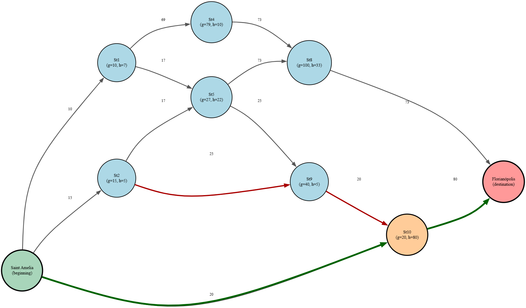
This is precisely why Street 10 (St10), despite having a relatively low edge cost (20), presents $h = 80$: geographically, it is far from the final destination. Meanwhile, Street 9 (St9), with $h = 5$, is well-positioned relative to Florianópolis, making it a more promising choice from the perspective of total estimated cost.
Therefore, the heuristic functions as a probabilistic compass: it does not guarantee the exact path, but guides the algorithm in the right direction, preventing it from wasting processing power exploring routes that are, geometrically, heading in the wrong direction.
The Two Lists: Open and Closed
The A* algorithm works with two lists:
- Open List: nodes that are known but not yet processed
- Closed List: nodes that have already been processed with defined cost
At each iteration, the algorithm selects the node with the lowest $F(n)$:
This node is removed from the open list and moved to the closed list.
With a consistent heuristic, the closed list is never revisited — it contains nodes already processed with the best known cost at that moment. Without consistency, it may be necessary to reopen nodes.
The open list, on the other hand, is constantly reorganized, prioritizing the lowest $F(n)$.
Important: if a node already exists in the Open List with a lower $g$ cost, we ignore any new path with a higher $g$. This ensures we always use the best known cost at that moment.
Practical Step-by-Step Simulation
Let’s analyze in practice how this works. Imagine we have the following scenario: traveling from Santa Amélia to Florianópolis, the bus needs to take the best route — the fastest and most efficient.
For this, we will work with a vector and two lists. Not all streets have exits or lead us to the best path; some are blocked or have high and irregular traffic.
We represent our route as:
Where:
- R is the route
- SA is Santa Amélia (starting point)
- St is Street n
- (cost_edge, h) are the values associated with each node
- cost_edge represents the cost to reach that node (defined by the edge) from the previous one
- h represents the heuristic (estimate of remaining cost to destination)
In this route, St3, St6, and St7 have traffic that is practically stopped and do not have valid connections in the graph for this example, so they do not participate in the simulation.
The valid routes are:
Each one has its own connections.
Graph Connections
Edge Costs
Step-by-Step Execution
Iteration 1: Expand SA
We calculate F for each direct neighbor of SA:
- Open List: \(\text{\{ SA }\} \rightarrow \{(\text{St}_1, 17), (\text{St}_2, 20), (\text{St}_{10}, 100)\}\)
- Closed List: \(\text{\{SA}\}\)
SA enters the closed list with cost 0 — it is the starting point. The lowest F is St₁, so we expand it next.
Iteration 2: Expand St₁
- Open List: \((\text{St}_2, 20), (\text{St}_5, 49), (\text{St}_4, 89), (\text{St}_{10}, 100)\)
- Closed List: \(\text{\{ SA, St₁ }\}\)
The lowest F is now St₂.
Iteration 3: Expand St₂
St₅ already exists in the open list with $g = 27$ ($F = 49$). Since $27 < 32$, we keep 49.
- Open List: \(\{(\text{St}_9, 45), (\text{St}_5, 49), (\text{St}_4, 89), (\text{St}_{10}, 100)\}\)
- Closed List: \(\text{\{ SA, St₁, St₂ }\}\)
The lowest F is now St₉.
Iteration 4: Expand St₉
St₁₀ already exists in the open list with $g = 20$ ($F = 100$). Since $20 < 60$, we keep 100.
- Open List: \(\{(\text{St}_5, 49), (\text{St}_4, 89), (\text{St}_{10}, 100)\}\)
- Closed List: \(\text{\{ SA, St₁, St₂, St₉ }\}\)
The lowest F is now St₅.
Iteration 5: Expand St₅
St₉ is already in the closed list → we ignore it.
- Open List: \(\{(\text{St}_4, 89), (\text{St}_{10}, 100), (\text{St}_8, 133)\}\)
- Closed List: \(\text{\{ SA, St₁, St₂, St₉, St₅ }\}\)
The lowest F is now St₄.
Iteration 6: Expand St₄
St₈ already exists in the open list with $g = 100$ ($F = 133$). Since $100 < 152$, we keep 133.
- Open List: \(\{(\text{St}_{10}, 100), (\text{St}_8, 133)\}\)
- Closed List: \(\text{\{ SA, St₁, St₂, St₉, St₅, St₄ }\}\)
The lowest F is now St₁₀.
Iteration 7: Expand St₁₀
We use the best known g of St₁₀, which is $g = 20$ (direct path SA → St₁₀).
- Open List: \(\{(\text{St}_8, 133), (\text{FP}, 100)\}\)
- Closed List: \(\text{\{ SA, St₁, St₂, St₉, St₅, St₄, St₁₀ }\}\)
Iteration 8: Expand FP
FP is the destination. The algorithm terminates.
- Closed List: \(\text{\{ SA, St₁, St₂, St₉, St₅, St₄, St₁₀, FP }\}\)
Final Result
By tracing the path backward — from FP to SA, following each node through its predecessor with lowest $g$ — we obtain the optimal route:
Total actual cost (g): 100
What happened to the other paths?
Therefore, even though the heuristic of St₁₀ is high ($h = 80$) — which caused it to be deprioritized initially — the algorithm did not discard it. It remained in the open list and, when its turn came, revealed the cheapest path.
This perfectly illustrates the intelligence of A*: the heuristic guides the search, but the actual accumulated cost ($g$) is always considered, guaranteeing that the optimal path is found.
Important Note: The heuristic is not added to the final cost of the solution. It only composes the function $f(n) = g(n) + h(n)$, which is used to prioritize the expansion of nodes during the search. The actual cost of the route is given exclusively by $g$.
You can follow the journey on the Graph below:
The A* Algorithm in Pseudocode
This is exactly the logic applied in the process.
Heuristic Quality and Algorithm Performance
The heuristic (h) plays a fundamental role in the algorithm’s performance, as it guides the search toward the objective. However, A* does not depend exclusively on it to function correctly:
-
If $h(n) = 0$ for all nodes: A* reduces to Dijkstra’s algorithm, still guaranteeing the optimal path, but with greater computational cost.
-
If the heuristic is admissible (never overestimates the actual cost): A* maintains optimality.
-
If it is inconsistent or overestimates: The algorithm may lose the guarantee of finding the best path.
Therefore, the heuristic does not define how the algorithm works, but rather its efficiency.
Computational Complexity
The complexity of A* in the worst case is:
Where:
- b = branching factor (average number of neighbors per node)
- d = depth of the solution
This means the growth is exponential with respect to depth. Although the branching factor directly impacts the number of nodes explored, depth has the most critical effect on total growth, since the number of nodes grows approximately as:
In other words, the cost is dominated by the deepest levels of the tree.
Conclusion
The A* algorithm represents a significant evolution in pathfinding. It combines the proven principles of Dijkstra’s algorithm with the intelligent guidance of heuristics, creating a method that is both optimal and efficient. The algorithm’s brilliance lies in its ability to balance two competing objectives: exploring the most promising paths (guided by the heuristic) while never discarding potentially optimal solutions (maintained by the actual cost).
In practical applications like GPS navigation, game artificial intelligence, and robotics, A* finds the best route not by examining all possibilities, but by making informed local decisions that, collectively, guarantee the global optimum. The bus driver leaving Santa Amélia will follow Street 10 directly to Florianópolis, bypassing congested streets entirely.
Every time a video game character finds the quickest path to their destination, every time a drone calculates the most efficient flight path, every time a logistics company optimizes delivery routes — the mathematics of A* is working behind the scenes, proving that a good heuristic combined with rigorous cost accounting produces excellence in problem-solving.