You are driving through the city, need to quickly get to a meeting with your girlfriend, and certainly don’t want to seem uninterested — delays can seem unforgivable. Luckily, you can always count on a routing app like Google Maps. But how does it actually work? If you had no app, just your paper map, how would you calculate the shortest route, considering the thousands of turns, hundreds of streets, and local and global variables? It can actually be done — though you’ll still prefer to use Waze.
The Problem
For this task we need an algorithm that allows us to go from point A and reach point Z in the shortest possible time. Although it seems simple, it isn’t. If the driver follows path $P = (v_1, v_2, \ldots, v_n)$, formed by a sequence of nodes, they can arrive at a given time $T$. However, to know whether this is the fastest route, they would first need to know the time of all possible paths.
Consider that each node in the route has $k = 10$ connections. The total number of paths grows exponentially: at each new depth level $n$ in the search, there are up to $k^n = 10^n$ possible paths to explore. With just 3 levels, that’s already 1,000 combinations; with 6 levels, we reach 1,000,000. In practice, since each connection leads to new nodes indefinitely, the search space grows without limit — making the brute-force approach computationally infeasible.
This would definitely not be fast or productive. The driver would follow path $(v_1, v_2, \ldots)$ and then $(u_1, u_2, \ldots)$, exhausting all combinations before even leaving the spot — and would still only be in the mapping phase. For this to work, they would need a complete map of the city with travel times for each route, which would already require excluding dynamic variables like traffic, making the result only a static approximation of reality.
Well, you might suppose that, if they have a map, they might know the distance between points A and Z, and that based on this they can metrically calculate the nearest kilometer. But here, it is necessary to understand that ordinary roads do not estimate time in kilometers — although they may be 2 km from their destination, they will still depend on the city’s routes and the availability of those routes. They may have to cross a stream along the way, and take a new, longer route.
Time and cost are defined in different ways, and, although even the driver may not know it, the cost of a path is formally defined as:
where $w(u, v)$ represents the weight associated with the edge between nodes $u$ and $v$.
Having understood the problem, we need to understand where the solution was born, how it emerged, and, most importantly, its algorithmic and mathematical foundations.
Dijkstra’s Algorithm
“What is the shortest way to travel from Rotterdam to Groningen, in general: from a given city to a given city. It is the algorithm for the shortest path, which I designed in about twenty minutes. One morning I was shopping in Amsterdam with my young fiancée, and tired, we sat down on the café terrace to drink a cup of coffee and I was just thinking about whether I could do this, and I then designed the algorithm for the shortest path. As I said, it was a twenty-minute invention. In fact, it was published in 1959, three years later. The publication is still readable; it is, in fact, quite nice. One of the reasons that it is so nice was that I designed it without pencil and paper. I learned later that one of the advantages of designing without pencil and paper is that you are almost forced to avoid all avoidable complexities. Eventually, that algorithm became, to my great amazement, one of the cornerstones of my fame.” — Edsger W. Dijkstra, in an interview with Philip L. Frana, Communications of the ACM, 2001 [1]
As we can see, a work of approximately twenty minutes yielded not only recognition for Edsger W. Dijkstra, but also fundamental applications in computing, GPS navigation systems, and artificial intelligence.
Initialization and Edge Relaxation
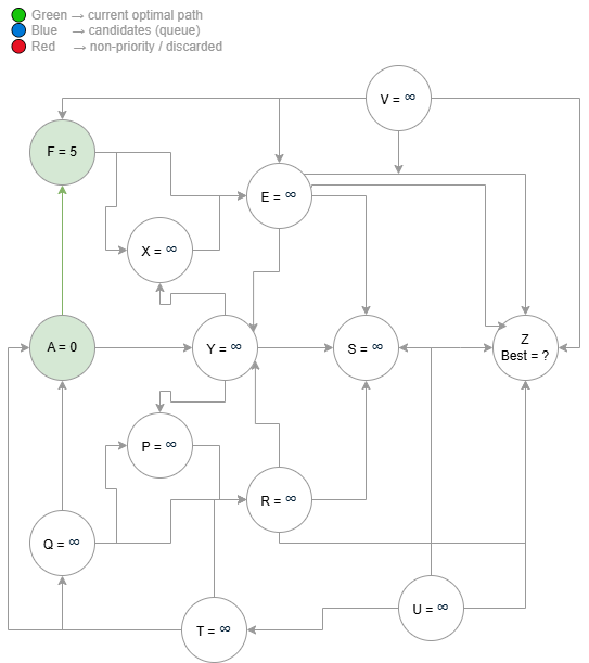
The algorithm requires an initial node — a well-defined starting point. For the late driver, this point is their current location, node $A$, and their goal is to reach $Z$ as efficiently as possible. Since they do not previously know the cost of all paths within a search space that grows approximately as $k^d$, it is initially assumed that all distances are unknown, represented as infinity [2]:
It is important to note that “cost” here does not necessarily refer to kilometers or Euclidean distance, but to the weight associated with the graph’s edges. This weight can represent travel time, road conditions, or any other relevant metric. The goal is to minimize the total accumulated cost.
The set of nodes can be represented as:
where the subscript indicates the cost known up to that point.
The first step consists of selecting the unvisited node with the lowest current cost. At the beginning, this node is necessarily $A$, since it is the only one with a finite value. From $A$, its neighbors are analyzed. Suppose there is an edge between $A$ and $F$ with cost $5$. In this case, the cost to $F$ is updated as:
This process is known as edge relaxation and can be described by the following rule:
From this point, $F$ is no longer a node with infinite cost and now has a concrete estimate. The updated set becomes:
Graph Expansion
The algorithm must move on to the next node not yet visited — not in the sense of being completely unknown, but in the sense that its lowest cost can still be updated. The choice of this node is not arbitrary: the one with the lowest known accumulated cost at that moment is always selected [3].
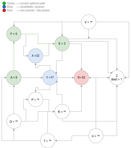
Suppose $F$ has been reached with $\text{dist}(F) = 5$. From it, the algorithm analyzes its neighbors, such as $E$, checking whether there is a better path through $F$:
This occurs because, for the driver to leave $A$ and reach $E$, they need to start from $A = 0$, reach intermediate point $F = 5$, and then continue to $E$, accumulating the total cost of the journey.
You might wonder how the algorithm determines the distance between each point. The answer is that it is fed with pre-defined data: the edge weights. In the driver’s example, the streets form the graph’s edges, while the neighborhoods represent the nodes. Thus, we can say that neighborhood $B$ is connected to others by different paths — $B \to C$, $B \to D$, $B \to E$ — each with an associated weight:
These weights can represent distance, time, or travel cost, estimated based on real data such as kilometers or traffic conditions. For example, although $B$ is 10 km from $Z$ in a straight line, there may be an edge $B \to C$ with weight $2$, representing a more accessible path within the urban network.
As the depth of exploration increases, the number of paths grows exponentially. Considering a branching factor $k$, the number of possible paths after $d$ levels is approximately $k^d$. It is this combinatorial expansion that makes it infeasible to determine the best path by simple inspection or manual trial.
Iteration and Convergence
Continuing the example, suppose the path $A \to F \to E$ results in a total cost [4]:
This means the best known path to $E$ has cost $8$. If a previous path already existed with a lower cost, the new value would be discarded, since the algorithm always maintains the lowest known estimate.
However, we have not yet reached $Z$. For this, the process continues from $E$’s neighbors:
Clearly more costly paths are not prioritized: if $\text{dist}(X) > \text{dist}(Y)$, $X$ is ignored and $Y$ is explored first.
Continuing from $E$ with $\text{dist}(E) = 8$, the algorithm explores its neighbors ${X, Y, P, Q, R, S, T, U, V, W}$, calculating:
| Node | Accumulated Cost |
|---|---|
| $X$ | $8 + w(E, X) = 40$ |
| $Y$ | $8 + w(E, Y) = 25$ |
| $P$ | $8 + w(E, P) = 50$ |
| $Q$ | $8 + w(E, Q) = 55$ |
| $R$ | $8 + w(E, R) = 65$ |
| $S$ | $8 + w(E, S) = 70$ |
| $T$ | $8 + w(E, T) = 100$ |
| $U$ | $8 + w(E, U) = 130$ |
| $V$ | $8 + w(E, V) = 180$ |
| $W$ | $8 + w(E, W) = 12$ |
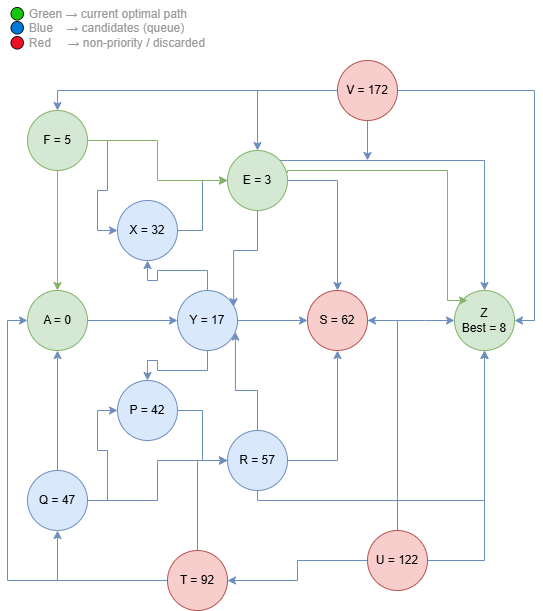
These paths are not discarded — they simply are not prioritized. The algorithm knows they may not be the best path, and therefore continues along the edge that indicates the lowest-cost route. The natural next node is $W$, since:
This process continues iteratively, always expanding the lowest-cost path until node $Z$ is reached. When this occurs, the value $\text{dist}(Z)$ will represent the lowest possible cost between $A \to Z$, regardless of the number of more costly alternative paths that exist in the graph.
Pseudocode
function Dijkstra(Graph, source A, target Z):

    // Initialization
    for each vertex v in Graph:
        dist[v] := ∞
        previous[v] := undefined

    dist[A] := 0

    // Priority queue of unvisited nodes
    Q := set of all vertices in Graph

    while Q is not empty:

        // Select the node with the lowest known distance
        u := vertex in Q with minimum dist[u]
        remove u from Q

        // Early termination upon reaching destination
        if u == Z:
            break

        // Explore neighbors of u
        for each neighbor v of u:
            if v is still in Q:
                alt := dist[u] + w(u, v)

                // Relaxation step
                if alt < dist[v]:
                    dist[v] := alt
                    previous[v] := u

    return dist[Z], reconstruct_path(previous, Z)


function reconstruct_path(previous, Z):
    path := empty list
    current := Z

    while current is defined:
        insert current at beginning of path
        current := previous[current]

    return path
The three diagrams below show the algorithm executing step by step over the same graph — from initialization through partial expansion to convergence at the optimal path.
Application in Real Systems
In systems like GPS, the balance is not based solely on kilometers. The edge weights incorporate environmental variables — traffic, road conditions, geolocation data. What the algorithm processes is not pure distance, but a composite cost that reflects the reality of travel [5].
In the example presented, the path found was $A \to F \to E \to Z$ due to the lower accumulated costs along those edges. However, this result is not fixed. Changes in weights can lead to completely different decisions. If $F$ is connected to multiple edges $F_1, F_2, \ldots, F_n$ with distinct weights, an imbalance in those values can turn a previously viable path into an inferior option, redirecting the search to another route.
The algorithm does not “choose” paths in a human sense — it responds directly to variations in weights. This is exactly what happens when you ignore Google Maps’ recommendation and decide to take a different route. In doing so, the system is not just “suggesting another route”: it is essentially restarting the calculation from a new state in the graph. Your new position becomes the new source node, and the algorithm recalculates accumulated costs for all possible paths — with the same weights, now potentially updated by variables such as traffic or road conditions.
Mathematical Formulation
The problem Dijkstra solves can be synthesized in one equation and one sentence [6]:
Find the minimum accumulated cost between a node $A$ and a node $Z$.
where:
- $\mathcal{P}(A, Z)$ = set of all paths from $A$ to $Z$
- $w(u, v)$ = weight of the edge between $u$ and $v$
- $P$ = a specific path in the graph
And the core of the algorithm can be reduced to a single operation:
Conclusion
The premises that make Dijkstra’s algorithm one of the most prominent for the shortest path problem from $A \to Z$ lie in the elegance with which it solves a complex question in a surprisingly simple way: comparing node weights systematically and always prioritizing the lowest known accumulated cost.
From a computational complexity standpoint, the algorithm’s performance depends directly on the data structure used for the priority queue. With a binary heap implementation, the complexity is:
where $V$ is the number of vertices and $E$ the number of edges in the graph. With a Fibonacci heap, this bound can be reduced to $O(E + V \log V)$ — relevant in dense graphs. In the most naive implementation, without a heap, the complexity is $O(V^2)$, which becomes prohibitive as the graph grows.
It is precisely this balance between correctness and efficiency that makes Dijkstra’s method applicable on a large scale. Every time Google Maps recalculates your route, every time a data packet chooses the most efficient path on a network, every time a game character finds the shortest route to their destination—there is, at some level, the same idea conceived in twenty minutes on the terrace of a café in Amsterdam. What Dijkstra did was transform a seemingly unsolvable problem into a sequence of simple, local decisions that, together, guarantee the global optimum.